2. Reading and writing

In hydrology, as in many scientific fields, reading and writing various types of data files is a fundamental task. Common file formats include binary files, raster data, CSV tables, and NetCDF datasets. Efficient handling of these formats is essential for performing large-scale or high-resolution analyses.

Before diving into file operations, it’s important to understand indexing in Julia, especially because many data formats (e.g., raster or NetCDF) are structured as multidimensional arrays.

2.1. Indexing

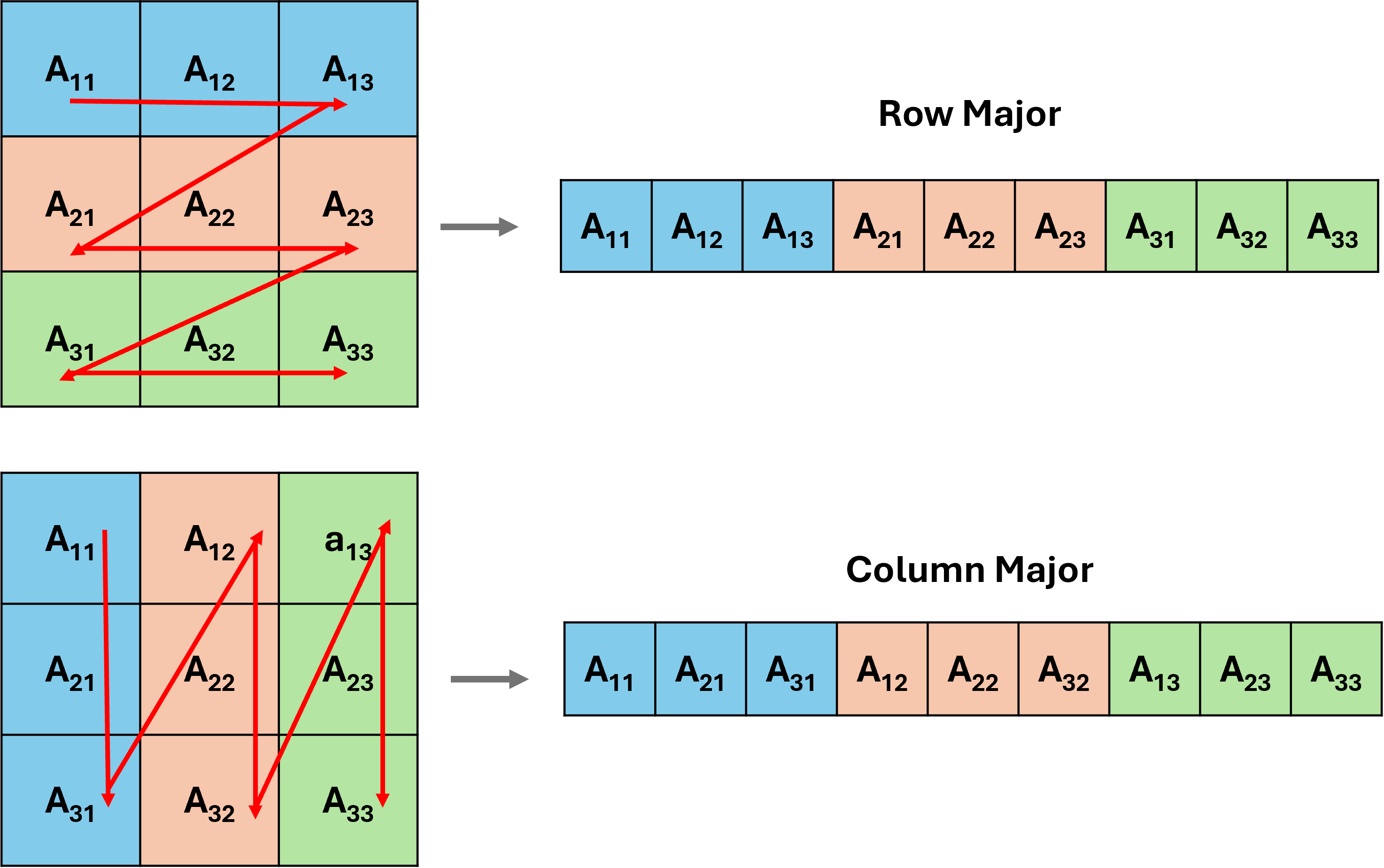
In Julia, arrays are one of the most commonly used data structures. Julia uses 1-based indexing, which is consistent with MATLAB and Fortran but different from Python or C, which start from 0. More importantly, Julia stores arrays in column-major order, which means that elements in a column are stored in contiguous memory locations.

This is particularly relevant when working with geospatial raster or multidimensional scientific datasets, as the order of reading and writing data (e.g., row vs column-wise) can affect both performance and accuracy (see Chapter 3 for details).

Understanding indexing helps when:

• Reading or reshaping data from binary or raster files.
• Mapping geographic coordinates to grid indices.
• Improving performance when working with large datasets.

Tips:

• When looping through arrays, prefer looping over columns (inner loop over rows) for speed.
• When reshaping binary data, match the shape and order to how it was written.

2.2. Binary Files

Binary files store raw data and are commonly used in hydrological models or satellite datasets for efficient storage. In Julia, you can read binary files using built-in functions such as open(), read(), and reinterpret().

# Example: Reading binary data
filename = "elevation_data.bin"
fid = open(filename, "r")
data = read(fid, Float32, (1000, 1000))  # Read 1000x1000 float32 grid
close(fid)

2.3. Raster Files

Raster files (e.g., GeoTIFF) are widely used in hydrology for storing gridded data like elevation, rainfall, or land use. Julia provides support for raster files through packages like GeoArrays.jl and ArchGDAL.jl.

Raster files typically include metadata such as:

• Coordinate Reference System (CRS)
• Geo-transform (mapping pixels to coordinates)
• No-data values

Understanding and preserving this metadata is critical for correct spatial analysis and visualization.

using GeoArrays

dataset = GeoArrays.read("dem.tif")          # Reading Tiff file
array = dataset.A[:,:]                       # reading as a matirx 

2.4. CSV Files

CSV (Comma-Separated Values) is a simple text format for tabular data, commonly used for time series, station metadata, or hydrological measurements.

Use CSV.jl and DataFrames.jl for fast and flexible parsing:

using CSV, DataFrames

df = CSV.read("streamflow.csv", DataFrame)
first(df, 5)

To write data

CSV.write("output.csv", df)

Tips:

• Always check for headers, delimiters, and missing values.
• Use Date types for time series parsing with DateFormat.

2.5. NetCDF Files

NetCDF (Network Common Data Form) is a widely-used format for storing multidimensional scientific data, commonly used in climate models, reanalysis, and remote sensing.

Use the NCDatasets.jl package:

using NCDatasets

ds = NCDataset("precipitation.nc", "r")
precip = ds["pr"][:]  # Read entire variable
time = ds["time"][:]
close(ds)

Why NetCDF is powerful:

• Supports metadata (units, dimensions, global attributes).
• Designed for time-varying multidimensional data (e.g., lat × lon × time).

Best practices:

• Always inspect metadata (keys(ds), attributes(ds[“var”])).
• Use slicing to load only needed chunks for large datasets.

2.6. Writing Data: Tips and Good Practices

• Binary: Use write() and ensure consistent dtype and shape.
• CSV: Use CSV.write() with DataFrames.
• Raster: Use ArchGDAL.create() with explicit CRS and transform.
• NetCDF: Use NCDataset(filename, “c”) mode to create and write.

Always document:

1. Units and data type
2. Coordinate systems
3. Time conventions (e.g., reference time in NetCDF)